This project models a chemical reaction where cold chemicals pour into a tank and react. It is based on papers of a number of authors beginning with R. Aris and N. R. Amundson in 1958 in the chemical engineering journals. We use data of Berger and Perlmutter from 1964. Scaling is a problem with most of the real data.
The reaction in the tank heats the chemicals and they pour out the other side of the tank at new concentrations. Some of the input chemical flows out the other side, but at a reduced concentration. That reduction has produced the substance we want to manufacture.
The reaction produces heat, but the cold chemical flowing in can absorb some heat. If it absorbs too much, the reaction stops. If it absorbs too little, things overheat. We want to know conditions for a stable equilibrium, in other words, conditions where the reaction continues at a stable temperature.
VARIABLES
We assume that the tank has volume V and is full from the start. This means that if chemical flows in at volume rate q (cubic feet/hr), then it also flows out at volume rate q. If the concentration of the chemical coming in is cin, then
THE AMOUNT OF CHEMICAL COMING IN PER HOUR IS
The concentration in the tank is c and it is flowing out at the rate q, so
THE AMOUNT OF CHEMICAL GOING OUT PER HOUR IS
One more thing happens to our input chemical: It reacts to form something else, thereby disappearing. The reaction rate depends on the concentration and the temperature.
48.2
Arrhenius' law says that amount of chemical disappearing per unit volume per hour is given by
We have used a number of parameters in the description and we need a few more.
Finally, we need to know the amount of heat generated.
Recall that Arrhenius' law says that the amount of reaction per unit volume is Ae-B/Tc, so there is a total amount of reaction VAe-B/Tc. The parameter H measures the rate of production of heat per unit of reaction, so
In short, we have found nonlinear differential equations of the form:
Measured parameters from the literature are:
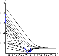
We will use the test case values for a sample computation. (The program TankReaction on our website is based on the text program Flow2D.) The flow of the differential equations in this case looks as in Figure 48.4.
Notice that there is an attracting equilibrium at a high temperature about 1.7 times the input temperature and another near the input temperature where
48.4
Our first job is to solve the equations for an equilibrium with the test case values of the parameters.
Next, we apply Theorem 24.6 of the main text.
We take
The program TankReaction on our website, based on Flow2D, may help you make a broader investigation of the tank dynamics.
Problem 48.1
48.5
Problem 48.2
Experiment on some unstable reactions to see how to run your cooler to stabilize them.

for constants A and B. The amount of chemical disappearing is thus VAe-B/Tc.

or that the rate of change of the concentration of the input chemical in the tank is given by

What is the parameter p?

THE AMOUNT OF HEAT GOING OUT IS 


and find the derivative of temperature with respect to time


where x=c and r=T/Tin.

where r=T/Tin and the computed constants are


Figure 48.1: A Flow Solution of the Tank Reaction Equations
 . The high-temperature equilibrium is using up most of the chemical and the low-temperature one is the case where the reaction has died out.
We want to find conditions that guarantee that the equilibrium that is using up input chemical is stable - neither explosively growing nor dying out.
We use Theorem 24.6 from the main text.

Your computer probably cannot solve these nonalgebraic equations exactly, so we begin with a plot of the implicit curves f[c,r]=0 and g[c,r]=0.


Horizontal and Vertical Vector Fields
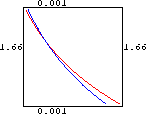
We used a numerical root-finding method to locate the three crossing points as follows: (0.992191,1.00521), (0.790976,1.13935), and (0.000917083,1.66606).

The characteristic equation is


and


are both negative if and only if both
 and
and
 are positive.
Investigate the reactions corresponding to the parameter values from the literature.
Suppose we could devise a cooling mechanism that sensed the temperature of the reacting chemicals and supplied cooling, say

Derive the new set of differential equations

where k[r]=K[rTin]/(TinsC) and recompute the stability conditions of the equations in terms of the new function k[r].