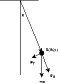
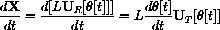
Figure 46.1: The Pendulum
The simple pendulum has been the object of much mathematical study. A device as simple as the pendulum may not seem to warrant much mathematical attention, but the study of its motion was begun by some of the greatest scientists of the 17th century. The reason was that the pendulum allows one to keep time with great accuracy. The development of pendulum clocks made sea travel safer during a time when new worlds in the Americas were just being developed and discovered. The scientist Christian Huygens studied the pendulum extensively from a geometric standpoint, and Issac Newton's theory of gravitation made it possible to study the pendulum from an analytic standpoint, which is what we will do in this project. The compound pendulum is still studied today because of its complicated "chaotic" behavior.
A simple pendulum is a small mass suspended from a light rigid rod. Ideally the mass will be small enough so that it will not deform the rod, but the rod should be light so that we can neglect its mass. (We will consider what happens if the rod stretches later in the project.) If we displace the bob slightly and let it go, the pendulum will start swinging. We will assume at first that there is no friction. In this idealized situation, once the pendulum is started, it will never stop. The only force acting on the pendulum is the force of gravity.
46.1
The force acting on the pendulum can be broken into two components, one in the direction of the rod and the other in the direction of the pendulum's motion.
If the rod does not stretch, the component directed along the rod plays no part in the pendulum's motion because it is counterbalanced by the force in the rod.
The component in the tangential direction causes the pendulum to move.
If we impose a coordinate system centered at the point of suspension of the pendulum and let
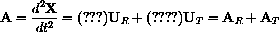
We will use the vector form of Newton's law, F=mA, to determine the equation of motion of the pendulum.
We assume that the origin of our fixed inertial coordinate system is at the pivot point of the pendulum shown in the figure.
The axes have their usual orientation.
Show that
The next step in finding the equations of motion of the pendulum is to use some basic vector geometry.
The gravity vector is simple in x-y coordinates, but we need to express it in radial and tangential components.
You should be able to remember a simple entry in your geometric-algebraic vector lexicon of text Chapter 15 that lets you compute these components as perpendicular projections.
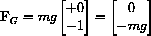
The magnitude of the gravitational force on the bob of mass m is mg and it acts down.
The constant g is the universal acceleration due to gravity (which we discussed in Galileo's law in Chapter 10.) g=9.8 in mks units.
As a vector, the force due to gravity is
The derivative of a general position vector with respect to t is the associated velocity vector.
The second derivative of the position vector with respect to t is the acceleration vector.
Calculate the second derivative of the position vector
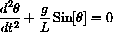
We can now use F=mA to determine the equation of motion of the pendulum.
We first need to note that the rod from which the bob is suspended provides a force that counteracts the radial component of gravity and prevents any acceleration in the radial direction.
Hence when we equate F and mA, the radial component of the acceleration is exactly balanced by the force of tension in the rod and the two expressions cancel.
Thus to determine the equation of motion of the pendulum we need only equate the expressions m times the tangential component of acceleration and the tangential component of gravity, mAT=FT.
Why doesn't the equation of motion for the pendulum depend on the mass? What does this mean physically?
46.2
In order to solve second-order differential equations numerically, we must introduce a phase variable.
If we let
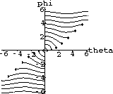
Figure 46.7 illustrates the phase plane trajectories of solutions to the system of differential equations for various initial conditions.
The displacement angle
Prove that
Make a contour plot of the function
Problem 46.1
Mathematical and Physical Experiments
As you can see from the phase plane there are two types of motion that the pendulum displays, the motion corresponding to the closed flow trajectories and that corresponding to the oscillating flow curves.
Explain physically what type of motion is occurring when the flow trajectories are closed curves.
Explain the type of motion occurring when the flow trajectories oscillate without closing on themselves.
Use the AccDEsoln program to plot explicit time solutions associated with each kind of flow line.
We suggest that you also try some calculations with various lengths.
A 9.8 m pendulum is several stories high and oscillates rather slowly.
It would be difficult to build such a large pendulum and have it swing through a full rotation.
How many seconds is a full oscillation (that is, what is the period)? How does the period depend on the length?
We suggest that you try some physical experiments as well, at least for small oscillations.
With small variations in
Problem 46.2
The Period of the Pendulum
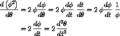
We would like to have a formula for the period, so we imagine the situation where we release the pendulum from rest at an angle
Compute the derivative
46.3
If the displacement angle
Problem 46.3
The Linearized Pendulum's Period
The true period of the pendulum differs from this amount more and more as we increase the initial release angle.
As you demonstrated above the period of the linearized pendulum is a constant independent of the initial displacement (and mass). This should give you some idea of why pendula are such accurate timekeepers.
If the pendulum is released at a certain angle to start and friction causes the amplitude of the swings to diminish, it still swings back and forth in the same amount of time.
In a clock, friction is overcome by giving the pendulum a push when it begins to slow down.
The push can come from weights descending, springs uncoiling, or a battery.
The comments about the invariance of period apply to the linearized model of the pendulum.
That model is not accurate for large initial displacements.
Another way to compare the periods is in the Flow2D solutions.
Compare the flow of the linearized model to the flow of the "real" (rigid rod frictionless) pendulum.
Why do the dots of current state remain in line for the linear equation and not remain in line for the nonlinear flow?
How nearly do the dots remain in line for the nonlinear flow under only "
How many minutes per month might you expect for a pendulum clock that has oscillations varying from 10 degrees fully wound to 8 degrees at the end of its regular winding period? Remember that the clock can be adjusted so that 9 degree oscillations would produce perfect time even though they do not have period
46.4
46.5
How would you modify the pendulum equation to account for friction on the pivot of the pendulum? How does this affect the accuracy of a clock? How would you modify the pendulum equation to account for air friction as the pendulum swings? How does this affect the accuracy of a clock?
46.6
Now we consider a mass suspended from a spring instead of a rod.
During the motion of the pendulum we will assume that the spring remains straight.
The force of gravity still acts on the mass and can be resolved into tangential and radial components.
There is also a force now due to extension of the spring.
If the spring remains straight it will act in the radial direction, but its effect is dependent on whether the spring is stretched or compressed.
Figure 46.18 illustrates the forces acting on the mass and their resolution into radial and tangential components.
In order to solve the system of second-order differential equations numerically, we must again introduce phase variables to reduce it to a system of first-order differential equations.
If we let y1=L,
Modify the AccDEsoln program to solve this system numerically.
Use g=9.8, L0=1.0, k=9.0, and m=1.0 for the acceleration due to gravity, the unstretched length of the spring, the spring constant, and the mass of the bob.
Start the pendulum by stretching the spring and giving it a small angular displacement.
For example, take y1(0)=2.5 and y3(0)=0.05. Use 0 as initial conditions for y2 and y4. How does the amplitude of the swings change as time goes on? In particular, does the amplitude of the swings increase, decrease, or remain unchanged?
 denote the vector giving the position of the pendulum bob, then Figure 46.1 illustrates the force of gravity on the pendulum and the resolution of this force into two components FR and FT.
Express the position vector
 of the mass in terms of the displacement angle
 , given that the length of the pendulum is L. Write X in terms of the unit vector
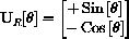
If the vector UR points in the direction of the rod, what are the directions of the x and y axes for the angle
as shown in the figure?

Prove that UT is perpendicular to the rod.
Prove that UT points tangent to the motion of the rod.
Sketch the pair UR and UT for
 . Draw UT with its tail at the tip of UR.
Decompose this vector FG into the two vectors FR, the radial component of gravity, and FT, the tangential component of gravity.
Express both vectors in terms of the vectors
 and
and
 defined above.
Verify that your decomposition satisfies
defined above.
Verify that your decomposition satisfies

for the scalar quantities you compute.
Show that the velocity of the position
 is given by
You can verify this by writing X in sine-cosine components or by using Hint 46.1.1.
 with respect to t and express the result in terms of the unit vectors UR and UT. You will need to use the chain rule and product rule in symbolic form, since the angle
 depends on t and we do not have an explicit formula for
 . Write your answer in the form
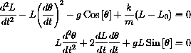
Equate these two expressions and use the formulas above to derive the pendulum equation: 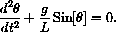
 , then the pendulum equation can be written as the system of differential equations:
This system can then be solved by the computer program AccDEsoln. Also, this system is autonomous.
Why? That means that we can use the Flow2D program to study the behavior of the pendulum.
What are the equilibrium points of the system above? Which equilibrium points are stable? Which are unstable? You should be able to determine this on purely physical grounds and then verify your conjectures with the comoputer. (What happens if you put the pendulum near the top?)
 is plotted on the horizontal axis, and the angular velocity
 is plotted on the vertical axis.
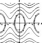
Figure 46.2: Phase Diagram for the Pendulum Equation
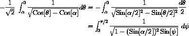
Calculate an invariant for the pendulum motion by forming the ratio

canceling dt, separating variables, and integrating.
 is constant on solutions of the pendulum equations.
 .
(HINT: See the main text, Section 24.4.)
.
(HINT: See the main text, Section 24.4.)
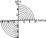
Modify the Flow2D program to build a flow solution of the pendulum equations.
We suggest that you use initial conditions (L=9.8 meter, g=9.8 m/sec2).
 = initxys = Table[{x,0},{x,-2 Pi,2 Pi,.6}] and
= initxys = Table[{0,x},{x,-2 Pi,2 Pi,.6}]
= initxys = Table[{x,0},{x,-2 Pi,2 Pi,.6}] and
= initxys = Table[{0,x},{x,-2 Pi,2 Pi,.6}]
 , a string will suffice for the rod.
These experiments are easy to do and you should measure the period of oscillation for various lengths.
, a string will suffice for the rod.
These experiments are easy to do and you should measure the period of oscillation for various lengths.
Verify physically and by numerical experiments that the period depends on the length but not on the mass.
 . For the time period while
 is a decreasing function, say one-quarter oscillation,
 , we could invert the function
 ,
,  . (See Project 21 and note that
 , so
, so
 .) Now we proceed with some more clever tricks.
Use the pendulum equation and integrate with respect to

Finally, separate variables and integrate to the bottom of the swing, one-quarter period,
This integrand is discontinuous at
 and may cause your computer trouble.
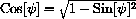
We do some trig,
and may cause your computer trouble.
We do some trig,
Now
with the change of variables
 and differentials
 , with
 when
when
 and
and
 when
when
 , using
 , we get finally,
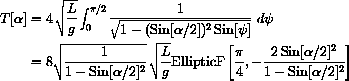
This is an "elliptic integral of the first kind," or in Mathematicajargon, "EllipticF." The integral cannot be expressed in terms of elementary functions, but the computer can work with this expression perfectly well.
See Figure 46.12 below.
 is small, then
 and we can approximate the pendulum equation by the simpler differential equation:
This is a second-order linear constant-coefficient differential equation and can be solved explicitly for given initial conditions using the methods of text Chapter 23.
Show that the period of the linearized pendulum is a constant
 .
. 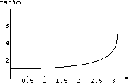
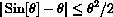
Figure 46.3: The Ratio

 and
and
 , solve the linearized pendulum equation symbolically.
What are the solutions if the pendulum has no initial angular velocity,
, solve the linearized pendulum equation symbolically.
What are the solutions if the pendulum has no initial angular velocity,
 ? From the explicit solution, determine how long it takes for the linearized pendulum to swing back and forth if it is displaced an angle
 and released.
Does the period of the pendulum depend on the angle
?
and released.
Does the period of the pendulum depend on the angle
?
Use the AccDEsoln program to solve the nonlinear pendulum equation for initial displacements running from 0 to
 . Use g=9.8 and L=9.8 for the acceleration due to gravity and the length of the pendulum.
The period of the linearized pendulum is a constant
. Use g=9.8 and L=9.8 for the acceleration due to gravity and the length of the pendulum.
The period of the linearized pendulum is a constant
 . How do the periods of the nonlinear pendulum compare to this constant? At what initial displacement does the linear approximation begin to break down? What happens if you vary the length?
Use the computer program Flow2D to solve the equations

with L=g=9.8 and initial conditions
 = initxys = Table[{0,x},{x,-2 Pi,2 Pi,.6}]
Nonlinear and Linear Pendula
The basis for our linear approximation to the equation of motion for the pendulum is the approximation
 .
.
Recall the increment equation defining the derivative

where
 if
if
 . Use this equation with x=0,
  and
and
 to give a first approximation to the meaning of "." In the Mathematical Background there is a higher order increment equation, Taylor's second-order "small oh" formula,

Substitute into this equation with x=0, , and
. Why does this give you a better approximation to the meaning of ""? The Taylor formula can be used to show that

Use this to show that
 . If a pendulum swings no more than
 , how large is the error between
 and
and
 ? What is the relative error compared to the maximum angle? How does this compare with the relative error of 1 minute per week? One minute per month?
Use the computer program Flow2D to solve the equations

with L=g=9.8 and initial conditions
 = initxys = Table[{0,x},{x,"
 ","
"," ",0.02}]
 " oscillations?
 .
.

Figure 46.4: The Spring Pendulum
 represent the position vector of the mass.
The length of the pendulum now varies with time.
Let L(t) represent the length of the pendulum at time t. Express the vector
in terms of L(t) and the unit vector
represent the position vector of the mass.
The length of the pendulum now varies with time.
Let L(t) represent the length of the pendulum at time t. Express the vector
in terms of L(t) and the unit vector
 defined above.
The force from the spring obey's Hooke's law.
If the unstretched length of the pendulum is L0, then the magnitude of the spring force is k(L(t)-L0), where k is the spring constant.
Express the spring force, FS, in terms of the unit vector UR defined above.
Resolve the force of gravity into radial and tangetial components, FR and FT as for the simple pendulum.
defined above.
The force from the spring obey's Hooke's law.
If the unstretched length of the pendulum is L0, then the magnitude of the spring force is k(L(t)-L0), where k is the spring constant.
Express the spring force, FS, in terms of the unit vector UR defined above.
Resolve the force of gravity into radial and tangetial components, FR and FT as for the simple pendulum.
 twice with respect to t to obtain the acceleration vector.
Express the acceleration vector in terms of the unit vectors UR and UT. Be very careful.
In this case both the length of the pendulum and the displacement angle are functions of t.
twice with respect to t to obtain the acceleration vector.
Express the acceleration vector in terms of the unit vectors UR and UT. Be very careful.
In this case both the length of the pendulum and the displacement angle are functions of t.
 ,
,  , and
, and
 , then the system becomes:
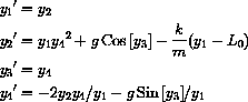
 and
and
 . If the ratio of these frequencies is a rational number like 1, 2, or
 , then the vibrations of the pendulum can exchange energies.
Change the value of k so that
, then the vibrations of the pendulum can exchange energies.
Change the value of k so that
 and use the same initial conditions as for the problem above.
How does the amplitude of the swings change in this case? Change k so that
and use the same initial conditions as for the problem above.
How does the amplitude of the swings change in this case? Change k so that
 and perform the same experiment.
Compare the amplitudes of the swings to the previous solutions.
Finally, change k so that
and perform the same experiment.
Compare the amplitudes of the swings to the previous solutions.
Finally, change k so that
 and perform the same experiments.
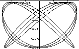
Figure 46.5: A Lissajous