Beddington's discrete dynamical model of Sei Whale growth is quite complicated. You need not try to justify it completely, but you should show that you understand what the main terms mean. We begin with an mathematical explanation of "carrying capacity" in terms of simpler models of population growth.
First, recall the discussion of algal growth in Section 3.3 of the main text.
The simplest equation describing the growth of a population is the exponential growth model, where the continuous time rate of change of the number of individuals is given by

for r defined as the per capita growth constant of the population. This model simply says that each "mother" N has "babies" at the continuous rate r.
The equation above describes instantaneous growth. It gives a good model of the initial growth of algae that are all reproducing at different times. Sei whales, however, birth a calf only once every 9 years, resulting in a "time lag" in growth. Moreover, they do this in a discrete "calving season." To represent this situation accurately, more complicated mathematics must be developed. We need discrete time steps to correspond to the calving season.
The differential equation is approximately

for time steps of size
 . In single unit time steps, this corresponds to the discrete dynamical system or discrete exponential growth law

The growth in the population from year t-1 to year t is p[t]-p[t-1], given by the term

This simply says that each member of the population p[t-1] at time t-1 gives birth to
 new members at the start of year t. (Typically,
 is a fraction, for example,
 means that each whale has one baby every 10 years, rather than a tenth of a baby each year.)
This model has the unrealistic feature that if
 , the population explodes to infinity (whereas if
 , the population cannot reproduce itself and becomes extinct.
The symbolic solution, given in Chapter CD20 of the main text, is the exponential function
 .) In the long run, such a model cannot describe actual populations - it tends to infinity and so would lead to overpopulation when
 . (Compare this with the results in the computer program ExpGrth from Chapter 28 of the main text, changing the 2 of the program to
 .)
.)
Overpopulation does not occur due to the limiting effects of food and space.
Another term can be added to the population growth equation that depends on the carrying capacity of the environment.
A simple "logistic term" gives us the discrete time equation

with the per capita growth

The parameter k is the mathematical counterpart of the environment's carrying capacity for the population. If p[t-1] is small compared with k, then
 and the per capita growth is approximately
 . As p[t-1] becomes closer to k,
  , the fraction
 , so the expression for per capita growth
 tends toward zero, stopping the growth.
If p[t-1] becomes bigger than k, then
 is negative and the population declines.
Example CD20.3 and Exercise CD20.4.2 in the main text show that the simple logistic system stably approaches the carrying capacity when
 and the initial population is not too far from k.
Beddington's model has the nonlinear term

that is analogous to the logistic term. When p[t-9]=k, this term is zero.


with k=26. This model is similar to Beddington's model, but without the 8-year delay in births. Use FirstDynSys for experiments and apply the conditions of Theorem CD20.4 to test symbolically for local stability.
42.2
The actual environment's carrying capacity for Sei whales needs to be measured in the actual environment.
That value becomes the value of k in our model.
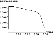
Our estimates of the past population of Sei whales is contained in the program WhaleHelp. A plot of that data is shown in Figure 42.3.
Beddington's model describes the whale population p at time t as a function of time.
It does this by giving a discrete dynamical system for p[t] in terms of p[t-1] and p[t-9]. The new feature here, compared with Chapter CD20 of the main text, is that births depend on the population 9 years ago.
It takes that long for a Sei whale to birth a calf.
Estimate the carrying capacity from Figure 42.3 (or the data in WhaleHelp). You will use your estimate as k in the model.
Here is a test case to use in helping us set whaling quotas from the model.
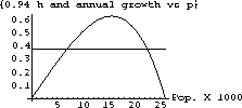
Suppose there is no hunting and the population has held at a constant level for 9 years, p=p[t-1]=p[t-9], what is the total change in the annual population for next year? Use the computer to plot the (unhunted) annual change as a function of p=p[t-1]=p[t-9] for values of p from 0 to 1.2k.
Now, consider the case in which the harvest levels are set
It is important to find the maximum sustainable yield.
When hunting is set at that level, whalers get the most whales possible while maintaining a population that can be hunted in the future.
Biologists and mathematicians have found that modeling the population of marine organisms like whales is a very complicated, uncertain process.
The parameters cannot be measured accurately.
It is therefore hard to estimate the biologically maximum sustainable yield, as well as to test the validity of a given model.
For this reason, it has been suggested that the harvest quota should be set at a fraction of the mathematically maximum sustainable yield derived from a model such as this one.
Simply looking a decade or two down the road isn't sufficient to ensure that the population will survive over centuries.
The future of the Sei whale population is in your hands - you must determine how the population will be affected by various hunting levels, which should be described in relation to the maximum sustainable yield.
The following exercise is a suggestion for investigations that will be helpful in understanding the dynamics of the model.
In addition, you are encouraged to develop other explorations that will better characterize the Sei whale population's dynamics, and so provide more information on how the population may be saved.
Good luck, and happy hunting! May your great-grandchildren hunt the grandchildren of our friend the Sei whale and each sustain the other.

Figure 42.1: Estimated Sei Whale Population of the Indian Ocean

The parameter h in the last term represents the number of whales that are hunted in the year.
If h=1000 whales were hunted, 6% of these would have died of natural causes anyway, so we deduct only .94h. The parameter k is the environmental carrying capacity.

Figure 42.2: Natural Change versus P  . Suppose the whale stock reaches some hunted equilibrium value, pH<k. If the population is at this constant population, pH=p[t]=p[t-1]=p[t-9], it will remain at this level.
When this equilibrium exists, the corresponding harvest quota, h, is called a sustainable yield.
The maximum sustainable yield is then defined as the largest yield for which the function has a nonzero equilibrium value.

Figure 42.3: Change and .94 Hunting

