Begin your projects with the derivation of the equation governing the mechanical or electrical oscillators associated with the second-order equations
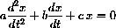
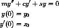
(Choose one or the other for your whole project.) In the case of a mass m attached to a spring with Hooke's law constant s and suspended in a damping material of constant c, this is just the Newton's law "F = m A" derivation of the core text. If y measures the weight's displacement from equilibrium, my" is the "m A" term, while the spring force is -sy and the damping force is -cy'. These forces are negative to reflect the fact that if you extend the spring to +y, it pulls back, etc. Draw a complete figure for your report and do the algebra necessary to put things in the final form
Derivation of the equation for an electrical oscillator consists of using current-voltage laws for resistors, inductors, and capacitors, then combining them with Kirchhoff's voltage law. One case is described in the project on the notch filter.
36.1
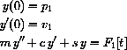
Your old e-homework program (core text Exercise 23.7.2) that solves the autonomous (also called homogeneous) initial value problems
You should include a few paragraphs of explanation on how the program works and why the various cases arise by assuming an exponential solution.
In other words, review the basic theory for your engineering manager, who may be a little rusty on these facts.
Give examples where the system oscillates and where it does not.
The computer program SpringFriction shows the result of lowering friction.
You may use it or excerpts in your report as long as you explain what the excerpts mean.
Give a careful explanation of the symbolic solution of the homogeneous problem above.
Be sure to include the mathematics associated with the interesting physical phenomenon of the onset of oscillation as damping friction decreases, causing the mathematical phenomenon of complex roots.
36.2
The solutions to the autonomous linear IVP are called transients, because they tend to zero as
If yT[t] satisfies:
This fact will play an important role in explaining the physical form of solutions to forced systems where the solutions "tend toward steady-state" as "the transients die out."
36.3
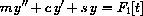
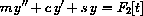
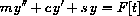
Imagine applying an external force to the end of the spring, F[t], besides the spring's restoring force and the friction -cy'. The resulting motion will be a solution to the nonautonomous differential equation
Also prove that if yS[t] satisfies
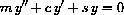
The (one and only) motion of the spring system is actually the unique solution to an initial value problem.
How can we formulate the superposition principle in terms of IVPs so that the mathematical solution is the physical motion? We either have to use special initial conditions or state the law in terms of steady-state solutions.
Include a mathematical formulation of the superposition principle in your report, explaining in very few words what this means mathematically.
There are several ways to do this.
36.4
We will begin with a very simple applied force, a constant.
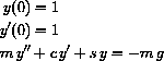
Suppose we hang our mass vertically on its spring and shock absorber (like a real car's suspension). The force due to gravity is mg and Newton's "F = mA" law becomes
What does the word "static" mean in this context? What is the derivative of your solution?
Recall that Theorem 23.7 of the main text says in particular that every solution of a homogeneous or autonomous second-order constant coefficient equation may be written as a linear combination of certain special exponential solutions.
That theorem is a computational procedure, but it guarantees that you find the one and only solution and you find it by solving for unknown constants in a certain form.
Conversely, if we let y[t]=yS+k1x1[t]+k2x2[t], for basic solutions x1[t] and x2[t] of my"+cy'+sy=0, then show that y[t] satisfies my"+cy'+sy=-mg.
Use the formula y[t]=yS+k1x1[t]+k2x2[t] to find a solution to
While you are solving this, think about how you would program the computer to do this for you and, more generally, how to program it to solve forced initial value problems.
You should include a program to solve these problems.
The commands in the electronic assignment Exercise 23.7.2 of the main text need to be modified.
The physical meaning of the previous exercise is that basic homogeneous solutions permit us to adjust initial conditions without disturbing the applied force.
The damping term, however, dissipates those "transient" solutions.
Show this.
36.5
Car suspensions are interesting only when we wiggle them.
As a test case, imagine an applied force that is a perfect sinusoid,
Conversely, if we let y[t]=yS[t]+k1x1[t]+k2x2[t], for basic solutions x1[t] and x2[t] of
As in the gravity solutions, the physical meaning of the previous exercise is that basic homogeneous solutions permit us to adjust initial conditions without disturbing the applied force.
That is all the homogeneous solutions do:
36.6
Use the formula y[t]=yS[t]+k1x1[t]+k2x2[t] to find a solution to
can be part of your project, but we want you to extend it to solve forced systems.
 . Transients don't stick around.
In Exercise 23.6.2 of the text, you showed that the fact that the constant c in the differential equation is positive means that any solution to the homogeneous IVP tends to zero. (We also showed this by an energy argument in Section 24.4, though you will probably find it easier to explain in terms of explicit solutions.) Include the solution to this problem in your projects:
. Transients don't stick around.
In Exercise 23.6.2 of the text, you showed that the fact that the constant c in the differential equation is positive means that any solution to the homogeneous IVP tends to zero. (We also showed this by an energy argument in Section 24.4, though you will probably find it easier to explain in terms of explicit solutions.) Include the solution to this problem in your projects:

with m, c, and s positive, then
 , no matter what initial conditions yT[t] satisfies.

Suppose that y1[t] satisfies
and y2[t] satisfies
Show that y[t]=y1[t]+y2[t] satisfies

and yT[t] satisfies

then y[t]=yS[t]+yT[t] still satisfies

and y2[t] satisfies
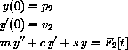
What initial conditions does the function y[t]=y1[t]+y2[t] satisfy; that is, what are the values of p3 and v3 in the following if y is the solution? 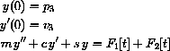
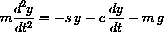
Show that the differential equation

does not satisfy the superposition principle.
Notice that x1[t]=t2 satisfies
 , that x2[t]=t2/4 satisfies
 , but that x1[t]+x2[t] does not satisfy
 .
.
when we measure y in an upward direction with y=0 at the position of the unstretched spring.
This is more simply written as

Find a simple formula for a constant solution yS=? to the above differential equation forced by gravity. (Hint: Plug a constant into the left-hand side.) Explain the formula for your solution in terms of the strength of the spring and weight of the object. (Which parameter measures spring strength?)
Suppose that y[t] satisfies my"+cy'+sy=-mg. Use simple reasoning and results from the course (which you cite) to show that we may write the solution in the form y[t]=yS+k1x1[t]+k2x2[t], for basic solutions x1[t] and x2[t] of my"+cy'+sy=0. (Hint: What equation does y[t]-yS satisfy?)
in the three cases m=1, s=1, c=3,2,1.
Show that every solution y[t] of
satisfies

by applying the exercise above and theory from the course.

We want you to find a solution by guessing a form and substituting it into the equation.
Assume that the solution has the form

plug yS[t] into the left hand side of the equation, tidy up the algebra, and equate coefficients on the sines and cosines.
You get the system of equations: 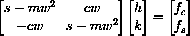
You can solve this with Mathematica's linear solve or use the 2 by 2 Cramer's rule: 
and the similar formula for k. We want to find an interpretation of this solution in terms of the limiting behavior of the system.
We will call the solution
 the "steady-state" solution for these particular values of h and k. We do not as yet know the actual solution that satisfies the initial conditions, but we do know Theorem 23.7 of the main text that tells us a form in which homogeneous solutions can be written.
Suppose that y[t] satisfies

Use simple reasoning and results from the course (which you cite) to show that we may write the solution in the form y[t]=yS[t]+k1x1[t]+k2x2[t], for basic solutions x1[t] and x2[t] of

(Hint: What equation does y[t]-yS[t] satisfy?)

then show that y[t] satisfies

Show that every solution y[t] of
 satisfies

by applying the exercise above and theory from the course.
What is the meaning of the limit? Notice that
 on the left-hand side, but not on the right.
How can we formulate this correctly?
on the left-hand side, but not on the right.
How can we formulate this correctly?
in the three cases m=1, s=1, c=3,2,1. While you are solving this, think about how you would program the computer to do this for you.
Extend your old e-homework program for homogeneous problems to solve the full problem (see the discussion following Hint 36.4.2 above): 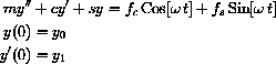
Combine the homogeneous and the steady-state solutions,

set t=0 in your program and solve for k1 and k2 just as you did in your program for the exact Mathematica solution of the homogeneous problem, but now take the initial value of yS(0) into account.