16.3 Drug Data
Figure 16.2 is a graph of blood concentration data similar to human data for the anticoagulant warfarin. (We could not obtain the raw data for a real human, so approximated them.) Our actual numbers are contained in the program DrugData on our website.

Figure 16.2: Warafarin Data
The data are given in a list of time-concentration pairs (t,c). These are entered in the form
data = {{.5,64.},{1,36.},{1.5,23.},{2,18.}, {3,14.},{4,14.},{6,12.},
{8,12.},{10,11.},{12,10.},{24, 8.},{36,6.},{48,4.0},{60,3.0}};
The times and concentrations can be separated as lists in Mathematicaas follows:
In[2]
{times, concens} = Transpose[data];
times
concens
Out[2]
{0.5, 1, 1.5, 2, 3, 4, 6, 8, 10, 12, 24, 36, 48, 60}
{64., 36., 23., 18., 14., 14., 12., 12., 11., 10., 8., 6., 4., 3.}
Once concentrations are separated, we can make a semilog plot as follows:
logCons = Log[concens];
logData = Transpose[times,logCons];
logPlot = ListPlot[logData,AxesLabel->"t","Log[c]"];
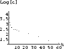
Figure 16.3: Log of Concentration versus time
Now we have the problem of guessing which points constitute the log-linear tail.
We can take the last eight data points as follows:
tail8 = Take[logData, -8]
These can be fit to a straight line by entering:
f8 = Fit[tail8,{1,t},t]
tail8Plot = Plot[f8,{t,0,60},AxesLabel->{"t","Log[c]"}];
Show[tail8Plot,logPlot];
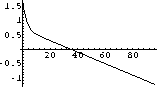
Fits for the last 8, last 6 and last 4 points are shown next:


: Linear Fits for 8, 6 and 4 Points
Problem 16.1
How many points should you use to fit the data to the linear tail? What are the various values of
 and h2 in the fits,

Once you have chosen
 and h2 from your best fit, you need to go back to the original data and remove the tail portion.
This can be done on the whole list with Mathematicaas follows:
In[19]
and h2 from your best fit, you need to go back to the original data and remove the tail portion.
This can be done on the whole list with Mathematicaas follows:
In[19]
h2 = 0.026
b2 = Exp[2.7]
remainders = concens - b2 Exp[ - h2 times]
Out[19]
{49.3125, 21.5022, 8.68941, 3.87424, 0.236777, 0.590009,
-0.730491, -0.0854228, -0.473041, -0.891689, 0.027485, 0.164266, -0.271649, -0.126768}
Problem 16.2
What is wrong with some of the remainders shown above? Can we take logs of the bad ones? What might have caused the trouble?
Our concentrations ideally are of the form

for the times in out list.
You have measured b2 and h2 the best you could from the data and computed the list of remainders.
Problem 16.3
As a function of t, what is the symbolic form of the remainders list?

Show that the symbolic form of the log of the remainders expression is a linear function
What are
 and h1 in terms of the parameters of the problem?
Ignoring the bad data for the moment, we can form the logs of the remainder data as follows in Mathematica:
headData = Transpose[{times,Log[remainders]}]
We can plot the first 6 points as follows:
headPlot = ListPlot[Take[headData,6],
AxesOrigin->{0,0},AxesLabel->{"t","Log[c]"}];
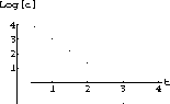
Figure 16.4: Six Points of
We can fit a line to the first four points as follows:
g = Fit[Take[headData,4],1,t,t]
headLine = Plot[g,t,0,4,AxesLabel->{"t","Log[c]"}];
Show[headLine,headPlot];

Figure 16.5: Linear Fit of the First 4 Remainder Points
Problem 16.4
The linear fit tells us b1 and h1. How?
Which is the best fit to the initial drop in concentration, the fit to 4, 5, 6 or 7 points?
Once you have answered this question, you know the approximate blood concentration function; for example, you might type:
b1 = Exp[4.8];
h1 = 1.7;
cA[t_] := b1 Exp[-h1 t] + b2 Exp[-h2 t];
cA[t]
curvePlot = Plot[cA[t],{t,0,60}];
Show[curvePlot,dataPlot];

Figure 16.6:  & Data
We could stop the project here, since we have measured the constants in the symbolic solution of the blood concentration.
However, it would be nice to connect our measured values of b1, b2, h1, and h2 with the physical parameters k1, vB, vT, k3, and cI, the initial concentration. (See Project 15 or Project 35 for the definitions of these parameters.)
% The initial dose of warfarin that produced the patient response of our data was the amount aI=100 mg. What is cB[0] with your measured values of b1, etc.? What is the ratio cI=aI/vB=100/vB? What is vB?
Two down, three to go.
Remember that k2=k1vB/vT.
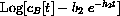
The Physical Parameters versus The Measured Constants
We are given that the ideal blood concentration is
where
1) Show that


 ) has a linear tail.
This is the starting point for our empirical work.
3) We also know measured values of h1 and h2, so compute k2 with both of the formulas above and find vT.
4) Above you showed that h1h2=k2k3, and now you know h1, h2, k2. Compute k3=?.
5) Above you showed that h1+h2=k1+k2+k3, and now you know h1, h2, k2, and k3. Compute k1=?.
6) Compute vT=?.
) has a linear tail.
This is the starting point for our empirical work.
3) We also know measured values of h1 and h2, so compute k2 with both of the formulas above and find vT.
4) Above you showed that h1h2=k2k3, and now you know h1, h2, k2. Compute k3=?.
5) Above you showed that h1+h2=k1+k2+k3, and now you know h1, h2, k2, and k3. Compute k1=?.
6) Compute vT=?.


 where
where
 . In other words, the slope -h2 is the rate constant associated with kidney function and the y-intercept is the log of the constant b2. This gives a way to measure b2 and h2 from data.
Once measured, if we subtract this measured part from the data, the resulting semilog plot is another line of slope -h1 with intercept
. In other words, the slope -h2 is the rate constant associated with kidney function and the y-intercept is the log of the constant b2. This gives a way to measure b2 and h2 from data.
Once measured, if we subtract this measured part from the data, the resulting semilog plot is another line of slope -h1 with intercept
 , corresponding to the fast initial drop.