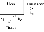
Figure 15.1: Two Compartments
Exponential functions arise in the study of the dynamics of drugs in the body. Here is a basic example. Suppose a drug is introduced into the blood stream, say by an intravenous injection. The injection rapidly mixes with the whole blood supply and produces a high concentration of the drug everywhere in the blood. Several tissues will readily absorb the drug when its concentration is higher in the blood than in the tissue, so the drug quickly moves into this second tissue "compartment." The kidneys slowly remove the drug from the blood at a rate proportional to the blood concentration. This causes the blood concentration to drop, and eventually it drops below the tissue concentration. At that point, the drug flows from tissue back into the blood and is continually eliminated from the blood by the kidneys. In the long term, the drug concentration tends to zero in both blood and tissue. The speeds with which these things happen is the subject of "pharmacokinetics."
Why should we care about such dynamics? Some drugs have undesirable, or even dangerous, side effects if their concentration is too high. At the same time those drugs must be above a certain concentration to be effective for their intended use. As the drug is eliminated from the body, doses need to be given periodically in order to maintain the threshold level for effectiveness, yet doses cannot be too frequent or too large or the concentration will exceed a dangerous level.
For now we just consider a single dose of drug that is introduced into the blood, diffuses into tissue, and is eliminated by the kidneys. Some of the drugs that fit the two compartment model are aspirin (acetylsalicylic acid); creatinine, a metabolite of creatine produced by muscle contraction or degeneration; aldosterone; griseofulvin (an antifungus drug); and lecithin.
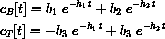
The concentrations in blood and tissue respectively are given by a linear combination of two exponential functions (sometimes called "biexponentials" in pharmacokinetics):
This project uses these formulas to understand the behavior of such a drug in the body. The Project 35, titled Drug Dynamics and Pharmacokinetics, has you show why the concentrations are given by these exponential formulas. The basic reason is that flow of the drug is described by simple differential equations. Project 16 shows how to use the ideas of this project to measure the dynamic parameters of a patient from data about blood concentrations.
15.1
Each drug and each patient have certain important constants associated with them.
In the complete story these will have to be measured.
15.2
Concentration is an amount per unit volume.
Suppose that a patient has 2.10 liters of blood and that 0.250 grams of a substance is introduced into the patient's blood.
When mixed, the concentration becomes
Suppose a patient has vB=2.10 and vT=1.30. If cB[t] and cT[t] were known functions, what would the amounts aB[t] and aT[t] be?
15.3
What we know from the theory in Project 35 is that
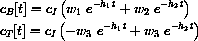
k1 = 0.17;
vB = 2.1;
vT = 1.3;
k3 = 0.03;
k2 = k1 vB/vT;
h1 = ((k1 + k2 + k3) + Sqrt[(k1 + k2 + k3)
h2 = ((k1 + k2 + k3) - Sqrt[(k1 + k2 + k3)
u1 = vT/(vT + vB)
w1 = (h1 - k2)/(h1 - h2)
u2 = vB/(vT + vB)
w2 = (k2 - h2)/(h1 - h2)
cB[t_] := cI (w1 Exp[ -h1 t] + w2 Exp[ -h2 t]);
cB[t]
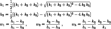
Notice that the blood concentration graph seems to have two parts: A fast decline followed by a slower decline.
What physiological things are associated with the fast and slow dynamics in the drug model? Which of the two exponentials decreases fastest?
Given that h1>>h2, if
Suppose t is fairly large, so that the fast exponential is negligible,
Show that the slope of the near-linear tail of the
How could you find b2 by extending the linear tail back to the cB axis?
Comparison of the model with data will require us to find where the linear tail in the semilog plot begins.
A clue is to compare the tissue concentration with the blood concentration:
The peak in the tissue concentration occurs just about at the end of the fast decline and the start of the log-linear decline.
We can find this time.
Compute this time for the specific constants w3, etc. coming from the model parameters k1, etc. where you have already graphed cT[t]. Compare this time with the peak on your graph.
The overall effect of a drug is related to the integral of cB[t] during the time when it remains above a minimum concentration for effectiveness, cE.
You may do your computation with the computer or the help of the program BiExponentialHelp on our website.
Then compute the numerical value of
Find two times t1 and t2 where
15.4
The mythical drug mathdorphin (MD) is produced in the body in large doses after a long period of serious effort on a difficult but interesting task.
When the concentration of MD in the brain exceeds 1 mg/l it produces a state of elated satisfaction.
Furthermore, the patient's IQ is noticeably increased in proportion to the period of time during which this excess concentration is maintained.
The amount of MD produced by the body is proportional to the square of the effort times the difficulty of the task.
Mathdorphin is released into the blood stream when a first submission of a project is handed in.
In this case the blood compartment consists of blood, liver, lungs, kidney tissue, endocrine glands, muscle, adipose, marrow, and skin.
A typical student then has a "blood" volume of 13.4 l. The "tissue" compartment consists of the brain and spinal compartment, where the important action of MD occurs.
The typical "tissue" compartment in this case is 2.31 l.
Through careful observation of students, we have collected rate parameters for a typical calculus student: k1=0.25 and k3=0.075.
Problem 15.1
Cumulative and Peak Effects of MD
MD does have one dangerous side effect.
If the concentration is maintained above 10 mg/l for more than 5 hours, the patient develops an irresistible urge to attend graduate school in mathematics.
Will you develop this neurosis? Try various initial blood concentrations and see how high this can go before you become a math nerd.
How much is your IQ increased?
15.5
 .
.
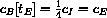
Give a general formula to convert the blood and tissue concentrations into the actual total amounts of the drug in the blood or tissue at a given time,

where cI is the initial concentration, or (dose/blood volume) and
These formulas give the exact symbolic unique solution of the full drug dynamics differential equations with initial condition (cI,0). They are messy formulas but amount to something that the computer can easily compute for us.
We want to get some sort of "feel" for the graph of such functions.
 2 - 4 k2 k3])/2;
 2 - 4 k2 k3])/2;
Graph cB[t] and cT[t] in case k1=0.17, vB=2.10, vT=1.30 and k3=0.03 and for several other choices of the parameters.
What is the general behavior of the graphs? Plot for a period of several days. (Note t is in hours.)
Graph
 in case k1=0.17, vB=2.10, vT=1.30, and k3=0.03. What is the general behavior of the graphs? Plot for a period of several days. (Note t is in hours.)


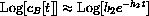
The first thing we can measure from data is the slow exponential.
This comes from the striking feature that you should observe in the semilog plot (or plot of
 ).
).
Why is h1>h2? (Hint: What is the formula for h2?)
 and t>>0, how does b1e-h1t+b2e-h2t compare with b2e-h2t? You could look at the sizes of both quantities or make the relative measurement and prove
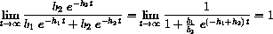
This limit says that for large t, the term b2e-h2t accounts for almost 100% of the concentration.
Why does it say this? In any case, explain why the term b1e-h1t accounts for the initial fast drop, while the term b2e-h2t accounts for the later slow drop and why the later part is mostly b2e-h2t.
 . What is the graph of
 for an interval of t values in this range? (Hint: Look at the previous figure and justify the graphically obvious feature of the tail of the plot.
Use
for an interval of t values in this range? (Hint: Look at the previous figure and justify the graphically obvious feature of the tail of the plot.
Use
 and
and
 ??.)
??.)
 graph is approximately -h2; in fact, the line has the form

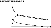
Figure 15.3: Twenty-four Hours of cB[t], cT[t], and

Let cT[t]=-w3e-h1t+w3e-h2t for positive constants w3, h1, and h2. Find the maximum of cT and show that the time where it occurs
Show that

and

Use numerical values of w1, etc. from the exact solution of the model for choices of the parameters to find the approximate time tE where
 . For example, use Mathematica's FindRoot[ cB[t] == cE , {t,3} ] or the program BiExponentialHelp on our website.
 . What are the units of the integral?
 . Why are there two such times? Then compute the numerical value of
 .
.
In the case of MD, the concentration in the brain must be held above 1 mg/l to produce the beneficial effect.
For each mg/l above 1 maintained 36 hours, the patient's IQ increases by one point.
How much smarter is this student after working this project?