3.2
3.3
As a warm up to magnifying graphs, think about this question: If you magnify a segment by one million and it appears to be 1 cm long, how long is it? We need a general formula to answer this kind of question so that we can predict when sufficient magnification will make a graph appear linear.
We begin with some numerics to help present the idea.
Finally, we want to compare the difference between these vertical distances.
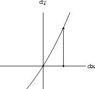
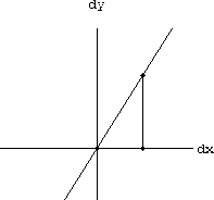
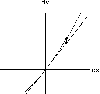
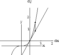
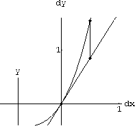
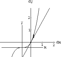
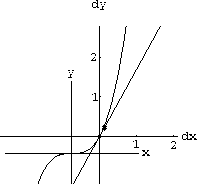
Figure CD-3.5 shows the nonlinear and linear graphs at magnification 8 and shows a small segment connecting the linear graph to the nonlinear one above
The error magnified by 8 (as shown) measures
In the following exercises, draw the sketches accurately on good graph paper.
Be careful about the method you use to calculate your results so you are connecting numerics, symbolics, and graphics.
You can use the computers if you wish, but you will still need to do algebra.
If you magnify by
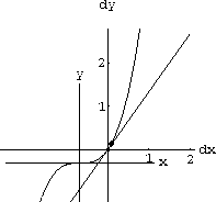
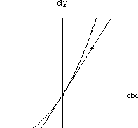
Your result from Exercise CD-3.3.2 should look something like the Figure CD-3.6. Compare your work to the computer animation in the program SecantGapZ.
Figure CD-3.7 is a sketch of a general function y=f[x] with 1unit=1cm. A pair of local coordinate (dx,dy)-axes is centered on the graph over a fixed point x. A line in local coordinates dy=mdx is shown in grey.
On the right, an image of these graphs is shown magnified by
Problem CD-3.1
Symbolic Magnification for an Unknown y=f[x]
3.4
The condition for local linearity of a graph y=f[x] is that the magnified error gap between the curve and line is small,
When the gap is small for
The condition of (uniform) "tangency" is expressed by the microscopic error formula
The approximation
When we say f'[x] is the derivative of f[x], we mean that this local approximation is valid,
Chapter 5 is devoted to symbolic computations of the gap
We expand
Show that no matter what magnification, we always have
Problem CD-3.2
To the right, the line has slope
We want to magnify this graph at (1,1) anyway and compare it with the "best" local linear approximation we can make.
Since the slopes average out to slope 1, compute the gap between this function and the line dy=dx.
Begin with several numerical cases.
Let x=1 and calculate
Graph the function and the line dy=dx on the same axes for the scales in the previous part of the problem and show that the gap remains the same size at all these scales.
Magnifying the graph never makes y=f[x] appear linear and never makes the gap between y=f[x] and dy=dx get smaller.
3.5
3.1.1
3.2.1
3.2.2
Section Summary
The goal of this section is to numerically and symbolically calculate the error of deviation from straightness in microscopic views of graphs.
 at
at
 ,
,  , magnification 8
The distance from the dx-axis to the point on the line dy=mdx above the point where dx=1/8 is

The magnified vertical segment at the right measures
 because we magnify by
 .
.
 . The actual length of the vertical segment connecting the (dx,dy)-point on the tangent with the (x,y)-point on the curve is the difference between these two values

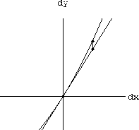
Figure CD-3.5: The magnified gap between y=f[x] and dy=mdx 
The moral of this whole chapter is that the error
 gets smaller and smaller as the x-increment,
 , gets smaller, even when we view this gap at magnification
 . This section only has some numerical examples to get us started at measuring this gap.
 , so that a segment of length
 appears to be unit size, and you observe another segment of apparent length
 , the actual length of the unmagnified segment is
 . The first exercise tries to help you understand this formula.
 and
and
 . Draw a line with a scale of 1 unit = 1cm on the left half of your paper.
Put dots at x=0,
  , and
, and
 . (What is the difficulty when you draw in centimeter units?) On the right half of your paper, draw a line starting at 0 magnified by 100. How far in centimeters on the magnified picture is the dot for
 and
and
 ?
?
 using equal x and y scales with 1 cm = 1 unit.
 at
at
 ,
, 
Carefully draw the curve y=x3 between the values
 and
and
 on a scale where 1/10 of a unit is 1cm, that is, magnified by 10 if 1cm is the original unit.
The curve y=x3 lies above your tangent line
 , where the local dx-dy axes lie at the center of the "microscope" magnifying the figure.
 , because dx=0 corresponds to
 What is the y-coordinate on y=x3 when
 ? What is the change in y from the dx axis to the point on the curve above x=2/3+1/10?
 ?
?
 on our centimeter scale is the magnified difference between the answer to Part 2 and the answer to Part 3, so its actual size is given by applying the formula from Exercise 1 to this difference.
How much is it?
Let f[x]=x3 in the following computations, and verify that the function procedures produce the answers to the measurement of
 as in the examples and exercises above, especially Exercise CD-3.3.3. Basic units are measured in centimeter, whereas magnified units appear 10 times larger.
 and
and
 with a scale of 1/10 unit = 1cm, the length of the vertical segment from the dx-axis to the (x,y)-point
 is 10 times the unit value of

or simply,

 is
is

If we magnify by
 so that
 appears unit size or specifically, 1/10 unit equals 1cm, then this distance measures

 measures

 is
is

3.3.2
Now we help you find the formula that expresses the quantities we see in a microscopic view of an unknown function y=f[x] when magnified by an arbitrary
 .
.
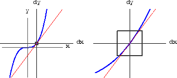
Figure CD-3.7: Slight magnification of y=f[x]  , so that the small number
 appears unit size.
Since we magnify by an amount that makes
 appear 1 cm in size, if we measure a distance
 in the microscopic image, the actual size is really
 . (Check this formula intuitively when
 . We magnify by one million and see a gap of 0.3, for example, but it is really only a gap of 0.3/1000000.)
Explain the following statements about Figure CD-3.7:

but the magnified view of this vertical segment measures

 is
is

but the magnified view of this vertical segment measures

 measures

but the actual change in the function as x moves to
 is
is

Section Summary
The following formula for the change in a general function

gives the gap
 one would measure at magnification
 between a straight line of slope f'[x] and the curve as we move from x to
 .
.  , when the magnification is large.
In other words, if the local change in x,
  , then the MAGNIFIED change along the curve is
 -close to the change along the line. (The lowercase [small] Greek delta ,
 , indicates intuitively that the difference in x is a very small amount.)
 , the slope of the local linear approximation, f'[x], is called the "derivative." This is what we saw in the examples and exercises of the last section:

provided the magnified error is small,
 , whenever the change in x is small,
 .
.
 means that a microscopic view of a tiny piece of the graph y=f[x] looks the same as the linear graph
 on the scale of
 . This looks like
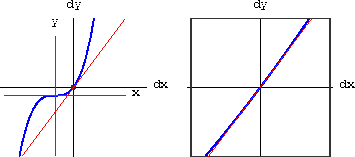
Figure CD-3.8: A Symbolic Microscope
 when
when
 , or
, or
 as
as
 .
.
 and symbolic ways to show that it becomes small when
 is small.
This is easy to verify in the case of y=x3.

with f'[x]=3x2 and
 . Because
 contains the number
 as a factor,
 is small when
 is small (as long as x is bounded.
See Chapter 5 for details.)
When f[x]=x3, the microscopic gap is
 .
.
 to check the errors you measured in Exercise CD-3.3.3 and Problem 3.3 .
 at x+1/100. How much is this gap when in a microscope of power 100 focused at the point x=2/3? How much is it really? Use your general formula to show that
 and
and
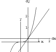
 (see Figure CD-3.9).
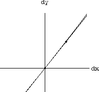
 at
at
 ,
, 
Let f[x]=x4 and show that the microscope equation

becomes

with
 .
.
 near x=0, but suppose the approximation we try is dy=dx, or m=1, so the microscope equation is

(see Figure CD-3.10).
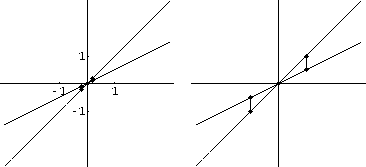
Figure CD-3.10: y=x/2 and dy=dx near (x,y)=(0,0), magnified
 5
5  above the point that appears to be one unit to away from the intersection. (Do this by writing f[x] and f'[x] explicitly in the microscope equation and solving for
 .)
.)
The graph of the function

is actually two half lines meeting at the point (1,1).
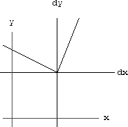
Figure CD-3.11:  near (x,y)=(1,1)
  , and to the left it has slope
 . There is no tangent line at this point because the "gap" does not go to zero. (Rules of differentiation from Chapter 6 applied to this formula give a formula that is not defined at x=1.)
 in the equation

for
 . (ANS:
  )
)
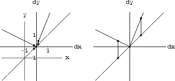
Figure CD-3.12:  near (x,y)=(1,1), magnified
 5
5
3.5.1
3.5.2
3.5.3
 and comparing it with the line
 in local (dx,dy)-coordinates centered at (x,y)=(3/4,27/64). We look at changes in x of
 and magnify each graph to look at the difference between the curve and the line.
We will make measurements in centimeters and adjust scales according to the amount of magnification.
 at x=3/4
 .
.
 at
at
 ,
, 
 at x=3/4
 .
.
 at
at
 ,
, 
 at x=3/4
 .
.
 at
at
 ,
, 
 , greek "E" (for error). In this example, we want to know
(1) How big is
 (in cm) in the microscopic view?
(2) How big is the gap in original unmagnified coordinates?Remember that if we magnify by one million and see 1 cm on the microscopic image, we actually have an error of 10-6 cm, one one millionth of the apparent error.
 is given by the difference,

 . The measured length after magnification is
 . The magnified linear approximation is shown at the right.