Linearity in function notation has a peculiar appearance.
This is not difficult, just different.
The exercises of this section give the linear case of the main formula underlying differential calculus,


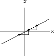
We want to consider the linear equation as a function, f[x]=mx+b, and compare perturbed values of the function symbolically and graphically. Some numerical computations may help get you started, but you should try to understand the fundamental role of the parameters m and b in general.
 and mark the point above
 on your graphs.
Each of your graphs should look something like Figure 9.1.
 appear on your graph?
i) Express your answer in terms of m, b, x, and
 .
.
ii) Express your answer in terms of f[x] and
 .
.
 into the formula for
 and show symbolically that

 in x is
 and does not depend on b or x. This formula could be expressed

 .)
.)


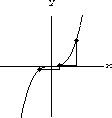
The important formula of the previous exercise is not true for nonlinear functions.
It fails in two ways.
Consider f[x]=ax2, for example.
If I say, "add 1 to x and tell me how much f changes," you can only answer in terms of x.


 symbolically and show that when we write the change in the function

 . (Hint: Compute
 .)
.)
The function f[x]=ax2 is smooth, so it satisfies the increment approximation

 when
when
 and f'[x]=2ax.

 is small.
Use your formula to explain: Why does the graph of y=ax2 appear linear on a small scale? Why does the slope of a microscopic view of the graph change when we chnage x?