Two lines are given by parametric equations as follows:

Find the distance between these lines; that is, minimize the distance between a point on line 1 and a point on line 2. Analytically, we have the question,
FIND: The minimum of |Y[s]-X[t]| for all values of s and t.
Since the square is an increasing function, we may as well solve the easier problem of minimizing the square of the distance

The partial derivatives of D are given by the chain rule

The critical point condition is the system of equations

with single solution (s,t)=(2,-1). The point X[2]=(2,0,0) is nearest to the point Y[-1]=(2,2,-1) at the distance
 .
.
Notice that the critical point condition for lines is a system of two linear equations in s and t. Solving this is a high school algebra problem.
You could use geometric or analytical reasoning to answer the last question.
Analytically, we could introduce a "fake" compact set for the (s,t) domain, say
 and
and
 with both S and T huge.
How large is D[s,t] on the boundary of the fake domain? Why does D[s,t] have both a max and min on the fake domain? Why is the min inside?
Example 31.1 Geometry of the Critical Point
The vector V pointing from X[2]=(2,0,0) to Y[-1]=(2,2,-1) is perpendicular to both lines,

The direction of line 1 is V1=(1,0,0) and the direction of line 2 is V2=(1,1,2)

Why must this perpendicularity be true?
- 1. Find the distance between line 1 in the direction (1,-1,1) through the point (0,1,0) and line 2 in the direction (1,2,1) through the point (2,2,2). Is the segment connecting the two minimizing points perpendicular to both lines?
- 2. Find the distance between line 1 and line 3 in the direction (1,2,1) through the point (2,1,2). Is the segment connecting the two minimizing points perpendicular to both lines?
- 3.
Let line
 be given by the parametric equations X[s]=P1+sV1 and line
 be given by the parametric equations Y[t]=P2+tV2. We want to minimize

Show that
Suppose that s0 and t0 are the critical solutions where these partials are zero. Show that the segment connecting X[s0] and Y[t0] is perpendicular to both V1 and V2,
(Hint: Substitute X[s0]=P1+s0V1 and Y[t0]=P2+t0V2 in the equations and compare with the partials.)


and solve them with the computer.
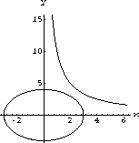
The computer's exact solution function may not be powerful enough to find exact solutions to the equations that arise from minimizing the distance between these curves, but the computer can approximate roots if you know a starting point. Look at Figure 31.4 above and say which roots are near the initial guess s=4 and t=2. Then calculate the result using a numerical solver such as Mathematica's FindRoot[ ] by making appropriate initial guesses. Remember that the computer can compute the partial derivatives for you as part of the solution program.
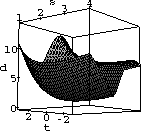
Use the computer to help you be sure you have what you need. For example, Figure 31.7 is a plot of the distance as a function of the parameters.

Figure 31.2: Distance versus (s,t)
31.3
We can work with the implicit equation of the ellipse and the parametric equation of the hyperbola.
First, we write the distance squared with a constraint,
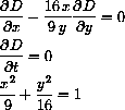
This differential is the local linear approximation to the change in the square distance function, so the critical values occur where it is the zero funciton.
Examples 19.9, 19.11, and the program SvVarMxMn from the main text find the distance from a point to a surface.
We can generalize those examples to find the distance from a line or a curve to a surface.
31.4
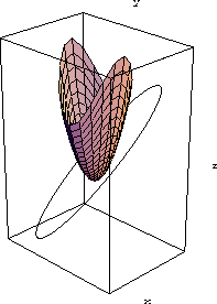
We generalize the main text Example 19.9 to find the distance between the explicit surface x3=x12+2x22 and the parametric curve
The squared distance function is
One solution we found was x1=0.979, x2=0.744, t=0.728. Is this the minimum distance?
Problem 31.1

We want to treat D as a function of x and t where y is determined by the constraint.


with your computer's numerical equation solver.
We got one solution x=2.053, y=2.917, t=2.827.


Figure 31.3: A Curve and Surface


You can easily invent any number of interesting distance problems yourself now and solve them with a combination of calculus and computing.

