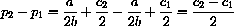
11.2
11.3
"Monopoly" means a manufacturer can choose whatever price she wants without fear of competition.
Our marketplace will be populated by a large number of individual consumers with no organized cooperation.
Their aggregate demand for the product will be determined by the price.
If the price is low, then the consumers will buy a great deal of the product.
But, as the price rises, the demand will fall.
Thus, the demand function will be some sort of decreasing function of price.
Our manufacturer wants to set the price that will maximize her total profit.
She cannot simply make the price as high as she wishes because demand will drop.
A high price on a few units may well produce less profit than a smaller price on many.
On the other hand, a very low price may sell many units but produce no profit because of the costs of manufacturing.
Our main simplification is in giving an explicit formula for the number of units of the product that consumers want to purchase or "demand." As an example, we begin by working with the linear demand function, D[p]=1000-500p.
Example CD-11.1
Maximum Profit for Demand D[p]=1000-500p
For this demand function, the maximum possible demand is 1000 units when the product is given away.
The maximum price is 2 dollars after which no one wants the product.
Thus, we are interested in a compact range of prices
Now, suppose that the manufacturing cost (i.e., raw materials and labor) for each unit of the product is 20 cents.
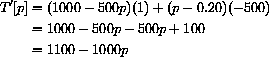
The unit profit at price p will be (p-0.20) and the total profit T[p] at the price p will be the number of units sold at the price p multiplied by the profit per unit.
In general, for any demand function D[p],
Our manufacturer wants to find the price p that maximizes her profit.
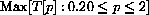
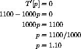
She wants to find the maximum of the function T[p]=(1000-500p)(p-0.20) on the interval [0.20,2]. We already know that the endpoints represent points of zero profit or the mathematically necessary, but economically uninteresting minima.
The next step is to differentiate the function T[p]. (We use the Product Rule rather than expand the expression.)
We have already seen that T[0.20]=0 (or T[0]<0) and that T[2.00]=0. There is only one critical point inside (0.20,2) so the Candidates procedure says the max must be at p=1.10, even without the slope analysis or the graph.
The profit maximizing price is
$ 1.10, and, at this price, the manufacturer will make a total profit of T[1.10]=405 dollars.
Example CD-11.2
A Parametric Maximum
You will notice an interesting phenomenon in the Exercise CD-11.5.3. Exactly half of the rise in the unit manufacturing cost is passed on to the consumer.
Is it true in general that a manufacturer always passes half of a cost increase to her customers? Let us begin by analysing a general linear demand function.
That is, use the demand function
Let the constant c represent the unit manufacturing cost for the product.
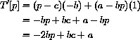
Thus, the profit per unit would be (p-c) and the total profit would be
Solving the optimization problem with the parameters a and b will tell us more than we would have known by solving only numerical examples.
The numerical examples suggested that half the cost increases were passed on in the linear demand case, but the parameter solution will show it.
Optimization with parameters often yields important insights beyond those that you can see from special numerical cases.
The parameters may be confusing so that working a numerical case helps to get started, but frequently they are indispensable for gaining scientific insight.
We want to find the profit-maximizing price as a function of the parameters.
The Candidates procedure says to check the endpoints and interior critical points.
We are to maximize T[p] over the compact interval [c,a/b], but we know that T=0 at the endpoints p=c and p=a/b. Hence, we calculate
This answers our question for any linear demand function.
If our first cost is c1, our first maximizing price is
What about nonlinear demand functions? See Exercise CD-11.5.4.
In Chapter 20, we investigate a dynamic model of price adjustment in an economy where producers do not have a monopoly.
Instead, they are willing to produce goods in quantities depending on the price.
That introduces the supply side.
11.6
Many max-min applications are easier to solve using implicit differentiation (first mentioned in Section CD-7.2). Review those simple examples to remind you how to use implicit differentiation and then we can apply the method to max-min with constraints.
Recall that the formula for the distance between the points with coordinates (x,y) and (a,b) is
This is simply a coordinate expression of the Pythagorean theorem that the length of the hypotenuse is the square root of the sum of the squares of the lengths of the two legs of a right triangle. (English is an awkward way to express this.)
Example CD-11.3
Points on a Circle Nearest a Point
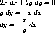
Find the points on the unit circle x2+y2=1 nearest and farthest from (1,1). We will use implicit differentiation in this basic example and ask you to generalize it and check your answer with common sense geometric reasoning in Problem 11.3.
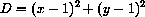
The distance from (x,y) to (1,1) is given by
Find
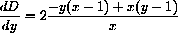
The differential of the square distance is
The differential of the constraint (when
Substituting this into the dy-expression in dD gives
The critical points where
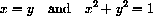
But the point must be on the circle, so we need to have both
Example CD-11.4
Endpoints in the Implicit Distance Problem
Once you see the solution to the previous problem on Figure CD-11.5, it is geometrically obvious.
However, there are two gaps in the reasoning we used and it is helpful to fill these gaps in a problem that is obvious.
First, we neglected the case y=0 when we computed the differential (since we divided by y.) In Chapter 19 we take a more geometrical approach (that does not require dividing), but, for now, we could simply solve the constraint differential for
The second gap in our reasoning is not just a technical problem.
Max-min theory works most effectively in the case where the independent variable of a smooth function runs over a compact interval.
In that case, we can guarantee that there is a max and a min and find them by checking endpoints and critical points.
Since we have given the problem implicitly, it is a little harder to justify use of this theory.
The variable x does range over the compact interval [-1,1], but we do not have the square distance given as a smooth function D=f[x]. We could apply the theory on the top and the bottom of the circle, where D=f[x] may be solved as a continuous function on a compact interval.
Those details show that there has to be a max and a min and that the critical values we have found are the only candidates. (A more systematic approach is given in Chapter 19.)
Solving the systems of equations that arise in constrained max-min problems can become quite technical, but do not forget the computer.
Example CD-11.5
Help from the Computer
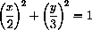
Find the points on the ellipse
SOLUTION:
The distance is given by
The differential of the squared distance is
The solution is shown on Figure CD-11.7. Notice the perpendicularity of the segments and tangents.
See Problem 11.3. This example is also solved using a parametric equation in Problem CD-16.5.1.
In this problem, we know that there is a max and a min because the variables x and y are confined to compact intervals, [-2,2] and [-3,3]. This is a little vague because the distance is not given by an explicit formula, but complete reasoning can be done along the lines of the circle example above.
Sometimes it is not so easy to see where the endpoint conditions enter a problem.
Here is another constrained maximization problem to illustrate this.
Example CD-11.6
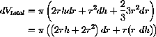
Hidden Endpoints A farmer wants to build a silo with cylindrical sides and a hemispherical top.
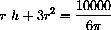
He has a fixed budget of 10,000 dollars.
The sides cost 3 dollars per square foot, but the top costs 9 dollars per square foot because of the labor and materials used in making it spherical.
What proportions should the farmer make the silo?
SOLUTION:
Draw a diagram of the silo and let the radius be r and the height h (measured in feet)
The area of the cylindrical side is
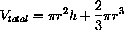
The volume of the cylindrical part of the silo is
The critical values,
This method obscures the role of endpoints somewhat because it does not make the dependence between h and r explicit.
We can reason that there are "endpoints" for r if we choose it as the independent variable, however.
First, if r=0, the silo has no volume.
The limit of Vtotal as r tends to zero should be zero, but this is not completely obvious because h must tend to infinity in order to hold the cost at 10,000 dollars.
However, the microscope comes to our rescue again.
The derivative
At the other extreme, if h=0 (so the silo is a hemisphere), you can still spend all the money.
Without solving, we can see that there is a maximal value of the radius.
Sometimes we can find extrema without calculus, and it is a good idea for you to compare a simple example with several methods.
Problem CD-11.1
A Geometric Minimum
Problem CD-11.2
Microscopic Geometric Minimum
The next exercise follows up on Example CD-11.3.
Problem CD-11.3
Another Geometric Minimum
11.7
We begin with a simple contrived example to illustrate how to work with a strictly symbolic max-min question.
Example CD-11.7
A Parametric Max-Min Problem
The function f[x]=x3+cx has a fixed but unknown parameter c. Find the maximum and minimum of this function for
First, the function is continuous everywhere because we can compute its derivative, f'[x]=3x2+c, by rules and a get formula valid for all real x. This means that the Extreme Value Theorem applies to f[x] on [-2,2]. The extrema must exist and, by the Critical Points Theorem, must occur either at endpoints or critical points.
Next, we want to know how the shape of the graph depends on the parameter.
Compute f'[x]=3x2+c and ask when the graph is level, f'[x]=0:
CASE 1: c>0
The number
At x=0, f'[x]=c>0, so the graph y=f[x] is always increasing.
This is the easiest case for max-min.
Since the function is increasing, f[-2] is minimal and f[2] is maximal for the x-interval [-2,2].
CASE 2: c<0
The numbers
At x=0, f'[x]=c<0, so the graph is decreasing near zero.
When |x| is huge, 3x2 is bigger than c, so the graph is increasing and the shape table is "up" before
The candidates for max and min are x=-2, x=+2 and the critical values, if they lie in the interval [-2,2]. Note that
The more interesting question in this specific case, however, is: When is the highest critical value greater than the highest endpoint value? By analyzing the shape table, "up" - "down" - "up", we want to solve
The minimum occurs at the negative value since the function is odd, f[-x]=-f[x], and the interval is symmetric
Here are some simple exercises on max-min with parameters.
Note that some are general cases of previous exercises.
We will see other important examples of the use of parameters in the following problems and in the projects.
The arithmetic mean is the usual average
Problem CD-11.4
The Arithmetic and Geometric Means
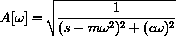
Resonance of a vibrating system is a maximal response to forcing.
Many old cars hum loudly at a speed like 46 mph, but are quieter at both slower and faster speeds.
The vibration at 46 mph is maximal, at least for an interval of frequencies (a local maximum). You can hear the resonance.
Cars with worn-out shock absorbers also oscillate.
In Chapter 23 we show that an idealized car's front end when forced with the pure sinusoid of frequency
Problem CD-11.5
Resonant Frequency of a Linear Oscillator
The idealized front end will oscillate on its own at a certain "natural frequency" when 4ms>c2. You do not get an interior maximum unless you have the condition 2ms>c2. Why is that?
The natural frequency is what you observe when a car with worn shocks goes over a bump and then back onto smooth (unforced) pavement.
The car keeps bouncing up and down for a long time.
This natural frequency is
11.8
11.5.1
11.4
11.5 Section Summary
In this section, we study simplified monopoly economies and show how a manufacturer maximizes profit.
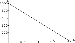
Figure CD-11.1: A linear demand function
 .
.

In this example

This further restricts the range of prices to
 because the manufacturer will not sell at a loss.
The next figure is a graph of this simple quadratic function.
because the manufacturer will not sell at a loss.
The next figure is a graph of this simple quadratic function.
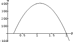
Figure CD-11.2: Total profit vs. price
Notice that she loses money to sell for less than 20 cents and that no one will buy for 2 dollars or more.
Next, we solve the equation
Thus, T'[p] is zero at p=1.10 and only there.
Notice, in addition, that T'[p] is positive if p<1.10 and T'[p] is negative if p>1.10. This means that the microscopic slope table is up-over-down, T[p] is increasing from p=0.20 to p=1.10 and decreasing from p=1.10 to p=2.00. Of course, we spoiled this analysis by showing the graph above first.
You can look at it to see the slope information.
We could have done the slope analysis without the graph - and might need to with a complicated demand function.

where a and b are arbitrary positive constants.
The graph of such a function, with D=a if p=0 and D=0 at p=a/b, is shown in Figure CD-11.3.
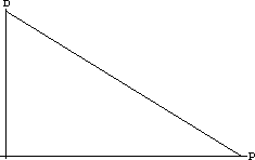
Figure CD-11.3: A general linear demand function

where a, b, and c are all positive constants.
To find the maximum, we set T'[p]=0 and solve
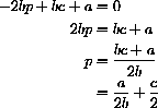
This price maximizes profit because some point must by the Extreme Value Theorem and there is only one candidate left. (You could make a slope table, up-over-down, turning at this price.)

If our second cost is c2, our second price is

and

(See Example CD-11.4 for the max-min analysis of this exercise.) Find the profit maximizing price in the following cases:
Section Summary
This section solves max-min problems with a constraint.
For example, we might want to know the minimum distance between two curves.
We are constrained to choose points on the curves.
11.6.1
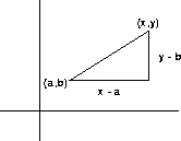
Figure CD-11.4: Coordinate Distance

 but we will maximize and minimize the square of this distance.
The square will be largest and smallest where the distance is, and differentiating the square is much simpler.
This makes our problem:
but we will maximize and minimize the square of this distance.
The square will be largest and smallest where the distance is, and differentiating the square is much simpler.
This makes our problem:


 ) is
) is
 (and
(and
 ) are:
We can easily solve these simultaneously, obtaining
 .
.
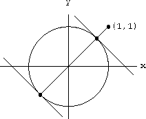
Figure CD-11.5: Points on x2+y2=1 nearest and farthest from (1,1) 
and substitute into dD, obtaining
Solving
 and the original ellipse equation gives the same answer when
 and we cannot have both x=0 and y=0.
that are nearest and farthest from the point (1,1). The distance from a point (x,y) to (1,1) is illustrated on Figure CD-11.6.
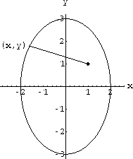
Figure CD-11.6: 
 , but it is easier to extremize the square,

and the differential of the constraint equation

is the equation
provided
 . We substitute this expression for dy into the differential dD, obtaining
so
and we have
 when the numerator is zero.
The numerator also involves y because we used implicit differentiation, so we must also satisfy the original ellipse equation.
The computer finds the simultaneous solutions of
when the numerator is zero.
The numerator also involves y because we used implicit differentiation, so we must also satisfy the original ellipse equation.
The computer finds the simultaneous solutions of

to be

[and two complex roots].
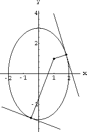
Figure CD-11.7: Points on
 nearest and farthest from (1,1)
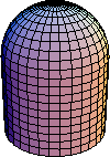
Figure CD-11.8: Silo
 , so the cost of the side is
 . The area of the hemispherical top is
 and its cost is
 . The sum is the total cost, which we set equal to
$ 10,000:
. The sum is the total cost, which we set equal to
$ 10,000:  , and divide both sides by
 to obtain
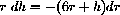
whose differential yields the equation

and
 , and the volume of the hemispherical top is
 , so the total volume is
with differential
substituting rdh=-(6r+h)dr, we obtain
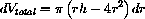
or
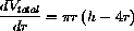
 occur at r=0 and h=4r. The answer to the question is that the height should be four times the radius.
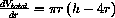 is positive when r is small and positive and h is large and the cost is fixed.
This means Vtotal increases for small values of r and cannot tend to a larger value than the one we found. (Can you write Vtotal explicitly in terms of r and find the limit of Vtotal as r tends to zero?)
is positive when r is small and positive and h is large and the cost is fixed.
This means Vtotal increases for small values of r and cannot tend to a larger value than the one we found. (Can you write Vtotal explicitly in terms of r and find the limit of Vtotal as r tends to zero?)
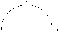
Figure CD-11.9: Rectangle inscribed in semicircle

Figure CD-11.10: Cylindrical can
Find the point closest to (x,y)=(1,1) on each branch of the hyperbola
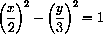
The computer says that the simultaneous solutions of

are
 and four complex roots.
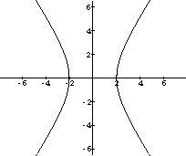
Figure CD-11.11: 
 and the point has coordinates (1,1). Find the coordinates of the point q. HINT: The equation of the line through p and q has slope 2 (the negative reciprocal of the slope of L) and passes through (1,1). Find the equation.
Make the algebraic statement that q=(x,y) lies on both lines and solve. .
and the point has coordinates (1,1). Find the coordinates of the point q. HINT: The equation of the line through p and q has slope 2 (the negative reciprocal of the slope of L) and passes through (1,1). Find the equation.
Make the algebraic statement that q=(x,y) lies on both lines and solve. . 
Figure CD-11.12: The distance from a point to a line
Suppose the point (x,y) minimizes the distance from a point (a,b) to a curve.
Why does the segment from (a,b) to (x,y) intersect the curve at right angles? (HINT: Imagine viewing the point (x,y) under a powerful microscope.)
Let a, b, and r denote constants.
Use calculus to show that the points on the circle

of radius r that are nearest and farthest from the point (a,b) lie on the line through the center of the circle and the point (a,b). Notice that the slope of the radial line from (0,0) to a point (x,y) on the circle is y/x and the slope of the line from (a,b) to (x,y) is (y-b)/(x-a). What is the slope of the tangent to the circle at (x,y)? Why does the equation
say that the segment from (a,b) to (x,y) meets the circle at right angles? Section Summary
This section looks at max-min problems with a parameter.
Often scientific max-min problems ask how the maximum depends on one or more parameters.
This is how Wein's Temperature Law is derived from Planck's Radiation Law in the projects.
Sharing half the cost of a price increase for linear demand was proved with parameters in the economics section of this chapter.
 .
.

Now, consider the cases: c>0 and c<0.
 is complex.
There are no real solutions to the equation: "y=f[x] is level"
is complex.
There are no real solutions to the equation: "y=f[x] is level"  f'[x]=0
  .
.
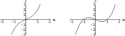
Figure CD-11.13: Examples of y=x3+cx with c>0 and c<0  are real - one positive, one negative.
The graph y=f[x] is level at these two points and nowhere else.
are real - one positive, one negative.
The graph y=f[x] is level at these two points and nowhere else.
 , "over" at
, "down" until
, "over" at
, "down" until
 , "over" at
, and up after that.
, "over" at
, and up after that.


 .
.
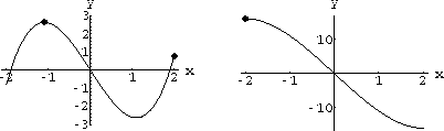
Figure CD-11.14: Examples of y=x3+cx with c<0 and c<<0 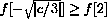 and find that this happens when
 . The maximum of f[x]=x3+cx for
 is at x=2; for
 , at
, at
 for
for
 ; and at x=-2 for
 .
.
 .
.
 where r is the radius of the cylinder and h is its height.
What should the dimensions of the can be in order to minimize the total area of the can and, hence, the cost of materials? (See Exercise CD-11.6.2.)
where r is the radius of the cylinder and h is its height.
What should the dimensions of the can be in order to minimize the total area of the can and, hence, the cost of materials? (See Exercise CD-11.6.2.)

The shape of the graph y=f[x]=2cx2-x4 for x>0 depends on the value of c. Which values of c give f[x] a positive maximum for
 ? (HINT: Find the critical values in terms of c. When are they real numbers? Prove your case by making a shape table as in Section CD-9.3.)

The geometric mean

is a sort of "multiplicative average" of positive numbers.
Also, notice that if
 and
and
 , then
 .
.

by squaring both sides and doing some algebra to put the inequality in the form


 is equivalent to

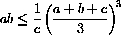
Treat a as a constant and use calculus to minimize the function
and show that the minimum is a when b=a. 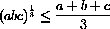
for positive numbers, with equality only if a=b=c. First, this inequality is equivalent to
so treat a and b as parameters and minimize the function
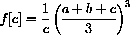
showing that the minimum is greater than ab, unless a=b=c when you get equality.
11.7.1
 ,
, 
has a response of amplitude
when it consists of a spring of constant s, a shock absorber with damping constant c, and mass m.
Find the maximum of
 for positive forcing frequencies
 . To simplify the problem, minimize the square of the denominator
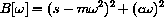
by showing that it has critical values at zero and the roots of a simple quadratic equation.
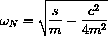
How does this compare to the maximal amplitude frequency (where B is minimized,
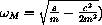 ? In particular, what happens in the particular cases

How do the frequencies compare when c is very small, that is, in the limit as your shocks become completely useless? What happens to the amplitude
 in this limit?
11.8.1
11.8.2
11.8.3