Advanced Calculus using Mathematica

Advanced Calculus using Mathematica: NoteBook Edition is a complete text on calculus of several variables written in Mathematica NoteBooks.

Local linearity: microscopic analysis of smooth quantities

A geometric interpretation of the tangent procedure is that the procedure computes what we would see in an infinitely (or “sufficiently”) powerful microscope.  The text has animations that let you increase the magnification in the following cases:

Zooming in on and explicit curve.

Zooming in on an explicit surface.

Zooming in on a contour plot.

Zooming in on a parametric curve.

Flow Increments.

Zooming in on a parametric surface.

Zooming in on coordinates in 2D

Zooming in on coordinates in 3D

Microscopic divergence and curl 2D

In Section 12.4 we show that flow along and across a small rectangle can be reduced to the linear vector field case because of the small oh approxiamtion:

, with ε≈0 when ,

Then we can break the linear term into cases and show the result of Green’s theorem by just geometry.  The sum of this result over a grid of small rectangles gives the integral Green’s formulas.

The Case shown with

The Case    shown  

The Case    shown with  

The Case    shown with

Microscopic divergence and curl 3D

The approach above for microscopic divergence in 2D works in 3D, but in Section 19.6 we take a different microscopic look at a vector field.  The linear approximation given by 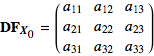   can be written as a sum of a symmetric matrix and an antisymmetric matrix:

The symmetric part,

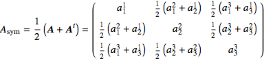
The antisymmetric part,

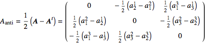
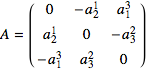, with 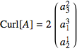and , by Exercise 2.

Zooming in on an flow equilibrium